Optimizers

• 24 Dec 2021
• 606 Views

Backpropagation is one of the techniques which is used to update the network’s weight to improve the performance of the model by minimizing the loss and making better predictions. The goal is to make the gradient descent move faster to the minima by avoiding the problems that can cause them to get stuck in different regions. Certain algorithms provide us the best learning rate to quickly converge to the minima. These algorithms are called as optimizers Avoiding the following surfaces are very important when it comes to gradient descent. Click here to learn Data Science in GNV IT Solutions

• Stochastic Gradient Descent with Moment

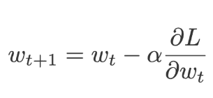
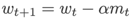
  Stochastic gradient descent picks the data point randomly from a dataset at each iteration which will reduce the computation. This gradient descent update the current weights by multiplying a constant value called learning rate, .

  

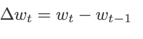
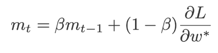
  When using SGD with momentum, for each iteration we will calculate the amount of change in the weight and then we add a small amount of its change from the previous iteration. The current weights are replaced by a momentum(m).Where momentum is the rate of change of current weights and previous weights.The value of m is initialized to 0.

  

  Where,

  

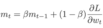
  β=0.9 (scaling factor)

• AdaGrad:

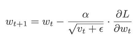
  Adagrad is called an adaptive gradient, as the name says the algorithm adapts the size of the gradient at each weight. It is applied to the learning rate which is divided by the cumulative sum of current and the previously squared gradients(v). Click here to learn Python in Hyderabad

  Because at each iteration the gradients are squared before its added, the value that is added to the sum is always positive. There is also a which is a floating-point added to ‘v’ just to make sure we will never come across a value divided by zero. This is called a Fuzz factor in Keras.

  

  Where,

  Watch Free Videos on Youtube

  

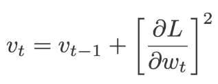
  The default values of α=0.01 and ε=10-7

• RMSprop

  The full name given to the RMSprop is Root mean square prop. RMSprop and Adadelta work on similar lines, RMSprop uses a parameter that controls how to remember. Unlike the Aadagrad where we take the cumulative value of squared gradients, the exponential moving average of the gradients is considered in RMSprop.

  

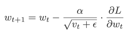
  Where,

  

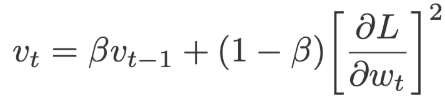
  The default values for:

  α=0.01, β= 0.9 (recommended) and ε= 10^-6

• Adadelta

  Adadelta is very similar to Adagrad but it has more focus on the learning rate. The full name of Adadelta is adaptive delta. Here the learning rate is replaced by the moving average of delta square values (delta is the difference between current and previous weights). Click here to learn Data Analytics in Hyderabad

  The values of v and D will be initialized to 0.

  

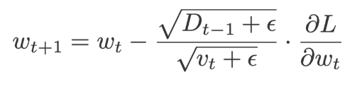
  Where,

  
  

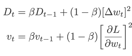
  The default values of ε= 10^-6, β=0.95, α=0.01

• Adam

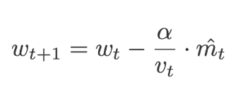
  Adam is called an adaptive moment estimation, it is obtained by combining the RMSprop and momentum. Adam adds the component m, i.e. the exponential moving average of the gradients to the gradient. The learning rate (α) is added by dividing the learning rate (α) with the square root of the exponential moving average of squared gradients(v). Click here to learn Artificial Intelligence in Bangalore

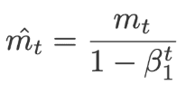
  The following equations are used to correct the bias,

  

  Where,

  

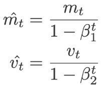
  And

  

  Where m, v is initialized to 0 along with

  α=0.001, β₁=0.9 and β₂=0.99 and ε= 10^-8

• Adamas

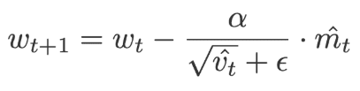
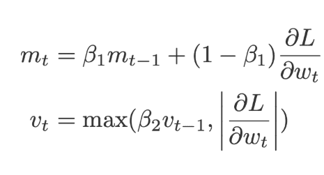
  Adamas is a type of Adam, these optimizers are used mostly in the models with embeddings. Here m is the exponential moving average of gradients and v is the exponential moving average of old p-norm of gradients which is then approximated to the maximum function. The following equation is used for bias correction. Click here to learn Artificial Intelligence in Hyderabad

  

  Where,

  

  And

  

  Where m and v are initialized to 0 along with

  α=0.002, β₁1=0.9, β₂=0.999

• Nesterov Momentum

  Momentum helps us get past information to get the network trained. But using Nesterov momentum it will reach us in the future.

  The ultimate idea is that instead of using gradients at a location where we are, we can use the location where we can be in the future. Click here to learn Machine Learning in Hyderabad

  It is like Momentum which utilizes the exponentially moving average m, where m is initialized to 0.

  It will update the current weights using the previous velocity.

  

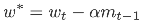
  This value is used to perform the forward propagation and the gradients are obtained for the same weights which are later used to compute the current weights(w) and the exponential moving average of squared gradients(v)

  

  Where β=0.9 and α=0.9 preferred.